Cleaning Football Data with R Tidyverse

Cleaning data is a big part of Data Science. Being able to script data cleaning makes it repeatable and transparent. The best tools to do this with in my opinion are R/Python/Power Query/SQL. In this post I take some scrapped Football data and clean it up with Tidyverse packages in the R stats eco-system. I've also created a basic Shiny app to show how this data can be further analysed.

The packages you need for this can be installed with tidyverse library(tidyverse).

First thing to do is load the CSV data into R memory.

Note, this is going into a Tibble data frame. Tibble is a modern data frame that is more strict, hence, easier to use.

setwd("/home/lee/Documents/Shiny/Football")
data <- as.tibble(read.csv("football_data.csv", header = TRUE))

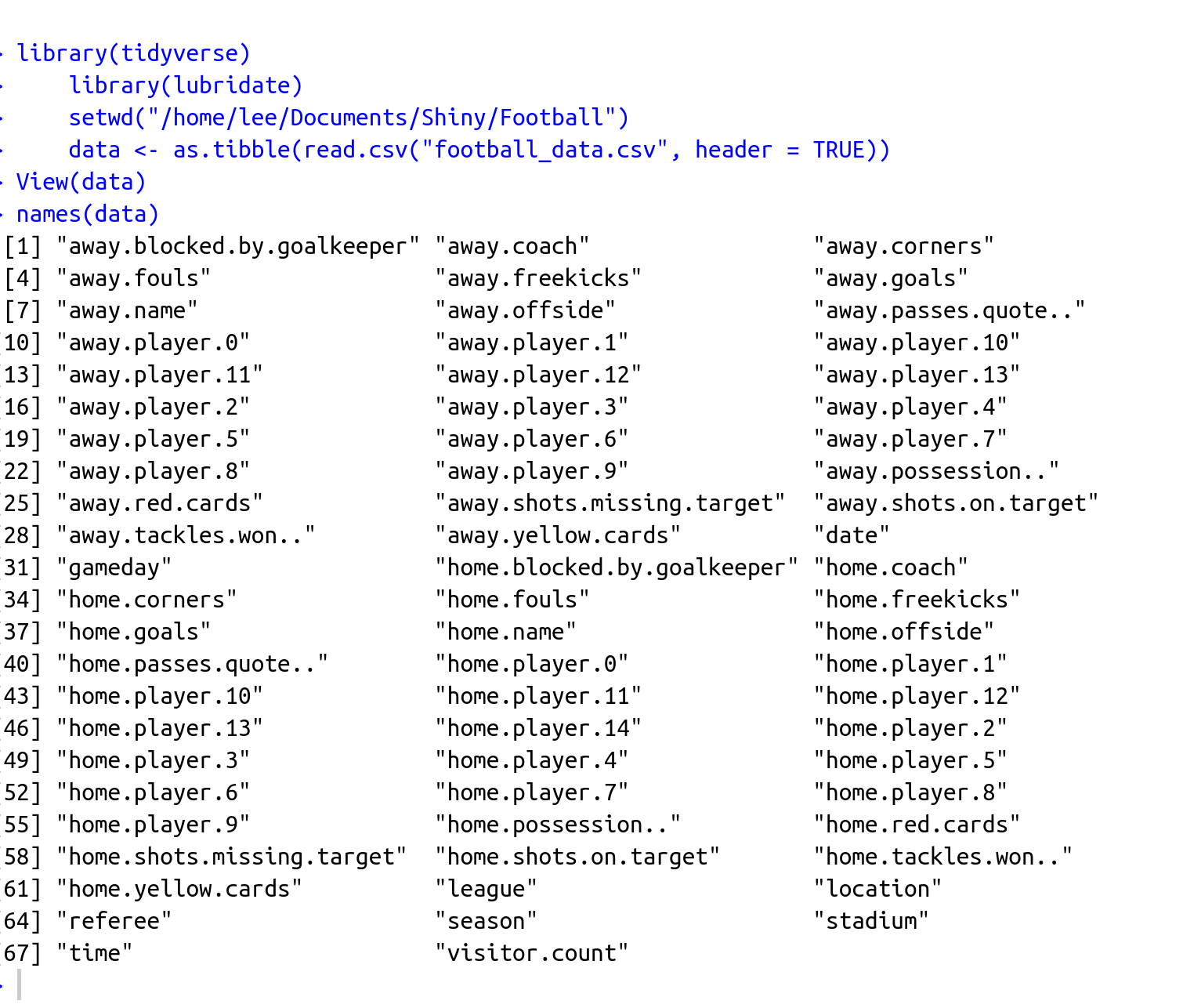
This data has many fields that I'm not going to use in this case.

There are around 27K rows as this data covers European football from 2005 to 2019.

So first step is to select the fields we're interested in.

We can use the Select() function to do this:

sub_data <- select (data,
                        c("away.player.0", "away.player.1",
                          "away.player.2", "away.player.3",
                          "away.player.4", "away.player.5",
                          "away.player.6", "away.player.7",
                          "away.player.8", "away.player.9",
                          "away.player.10","away.player.11", 
                          "home.player.0", "home.player.1", 
                          "home.player.2", "home.player.3", 
                          "home.player.4", "home.player.5", 
                          "home.player.6", "home.player.7", 
                          "home.player.8", "home.player.9", 
                          "home.player.10","home.player.11",
                          "home.name","away.name", 
                          "date", "league","home.name",
                          "away.name"
                        ))

I don't want the Players in rows in this case, hence, a pivot is required.

We can use Gather() to do this:

data_pivot <- gather(sub_data,key = "Field", value = "player",
                         "away.player.0", "away.player.1",
                         "away.player.2", "away.player.3",
                         "away.player.4", "away.player.5",
                         "away.player.6", "away.player.7",
                         "away.player.8", "away.player.9",
                         "away.player.10","away.player.11", 
                         "home.player.0", "home.player.1", 
                         "home.player.2", "home.player.3", 
                         "home.player.4", "home.player.5", 
                         "home.player.6", "home.player.7", 
                         "home.player.8", "home.player.9", 
                         "home.player.10","home.player.11"
                         
    )

This has exploded the rows to around 60K.

There's a little more data cleaning.

• Replacing the text date with an ISO formatted date.
• Adding a count field to help with analysis.
• Select the final fields.
• Filtering out blank rows from the Pivot operation.

final_dat <-select (data_pivot,
                    c("home.name", "away.name", "date", "league",player")) %>% 
            add_column(real.date=dmy(data_pivot$date), count=1) %>%
            filter(player !='') 
    
#Remove old date
final_dat <- final_dat[,-3]

Just a little cleaning up of the workspace left.

rm(data,sub_data, data_pivot)

There are lots of choices to make with cleaning. In this case I was interested in seeing Player data. If you wanted to see Match data there would be different cleaning i.e. probably no need for the pivot.

With R Stats we can publish apps quite easily with Shiny.

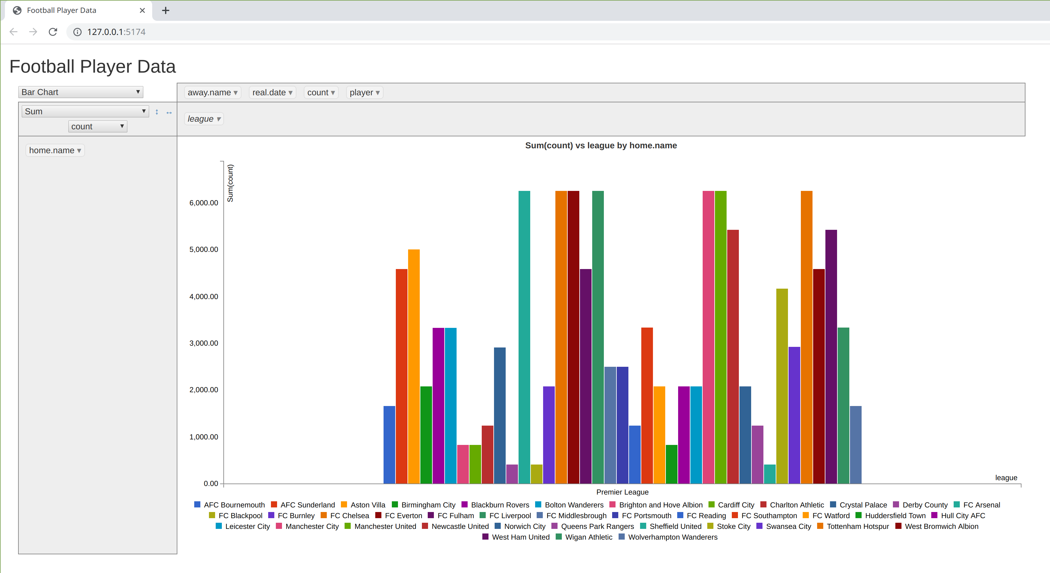
I decided to try out the RpivotTable package.

If you're new to Shiny we need to create a Server.R and UI.R script.

Here's my server.R code

library(shiny)
library(rpivotTable)

shinyServer(function(input, output) {
   
    output$pivot <- renderRpivotTable({
        rpivotTable(data = playerData(), rows=c("player"), 
                    cols="league", vals="Count", 
                    aggregatorName = "sum", 
                    rendererName = "Table", width="100%", height="500%")
    
        
    })

})

The UI data is very simple:

library(shiny)
library(rpivotTable)

shinyUI(fluidPage(

    # Application title
    titlePanel("Football Player Data"),

        mainPanel(
            rpivotTableOutput("pivot")
        )
    )
)

This creates a web based Pivot table that can be used to explore data.

Summary

There are many ways to skin a cat with R. The Tidyverse group of packages make this relatively straightforward.

Shiny provides for rapid development of data applications.

If you want to practice, some other actions that can be used to enhance the data :

• Add Year/Month fields
• Combine the Home / Away teams i.e. Liverpool FC vs Everton FC.
• Add statistics for Player performance

The CSV is available on Kaggle along with many other datasets.